Only a select few of my closest friends are aware of my journey from computer illiteracy to becoming a computer scientist. Recently, my very dear friend and my first mentor, Anshit Mandloi, encouraged me to pen a blog post about my progression—how I managed to transcend my lack of knowledge in computers and present my work at the Massachusetts Institute of Technology (MIT) within four years.

The purpose of sharing this deeply personal account is to provide inspiration to individuals who, like me, hail from similar backgrounds and may be grappling with doubts about their potential to navigate the vast landscape of technology. Through this blog post, my hope is to kindle the spark of possibility that with determination, the most remarkable transformations can be well within our reach.

The Beginnings

I come from a small town situated in one of the less developed regions of North India. Hailing from a family of eight, my father shouldered the role of the sole provider. In such circumstances, pursuing quality education proved to be an uphill battle, rendering the idea of having a computer at home an impossible dream. Hence, my exposure to computers was limited to the few sessions we had during our high school curriculum.

However, destiny had its designs, I managed to emerge successful in the IIT-JEE exam (an exam with an acceptance rate of 1%). This paved the way for my academic journey, leading me to opt for the study of Mathematics and Computer Science at the Indian Institute of Technology, Kharagpur.

The Challenges

IIT Kharagpur marked the beginning of a grueling trial. I very vividly recall my initial encounter with a black terminal screen, on a Sun Microsystems Unix machine, during my first C programming lab. Panic washed over me as I found myself completely clueless about navigating this challenge. For the first 30 minutes, I remained immobilized and it was only after summoning the courage to approach one of the teaching assistants and confess my utter inexperience with the computers that I got myself started. This was just the beginning of a huge challenge that lay ahead. As the clock ticked, I mustered the determination to engage with the terminal, but the initial hours only yielded a mere 2-3 lines of code. Some of my classmates, in stark contrast, efficiently accomplished the task within half an hour. Attending lectures with unwavering attention became my mantra, though comprehending the intricate subject posed a trial in itself. Even trying to read books like "The C Programming Language," authored by one of the language's creators, failed to yield substantial success.

It was, undoubtedly, a humbling experience to transition from being one of the top performers to grappling with a newfound identity as one of the class's less accomplished individuals—especially amidst peers who had participated in international programming olympiads.

What accompanied these challenges was not merely technical, but a roller-coaster of emotions. Frustration set in, and self-doubt crept in as I questioned my capability to bridge the gap between my knowledge and the complex world of programming.

The Journey

Over time, my determination to grasp the unfamiliar and uncover the secrets of programming only grew stronger. I began with a book that my professors discouraged but I could understand it on my own - "Let Us C" by Yashwant Kanetkar. My evenings were dedicated to the library, reading a page or two and writing down notes. Every week, I spent all my allotted lab time attempting assignments, often ending in failure.

It was during these moments that I found invaluable friends and mentors who recognized my need for help. My wingmates, Anshit Mandloi, and Naman Mitruka, were instrumental in my journey. They patiently listened, clarified my doubts, and even guided me through basic programming exercises.

In my second year at the university, I met Harsh Gupta, who was my batchmate, and he played a pivotal role in my growth as a programmer. His willingness to lend a helping hand on numerous occasions marked a turning point in my journey. He generously shared his knowledge, ensuring I grasped complex concepts and tackled intricate problems with confidence.

After three years of taking various courses, and participating in hackathons (with mostly failures), my confidence as a programmer began to bloom. It was finally time to put my skills to the test in the real world.

MIT

My aspiration was to become a part of the esteemed Google Summer of Code program. In my initial attempt at the end of my third year at university, I faced rejection. I tried the following year and my effort bore fruit. I spent the summer of 2016 contributing to the Julia Programming Language, specifically adding support for optimization with complex numbers in their Convex.jl library.

It was during this summer, an unexpected invitation arrived: I was asked to speak about my work at JuliaCon'16, hosted at MIT in Boston. Visiting MIT had always been a dream, one I thought might forever remain unfulfilled, let alone being invited as a speaker at a conference there. It felt as though all my struggles and hard work had unknowingly paved the path to MIT. This experience to this day still stands as one of the proudest moments of my life, reinforcing the belief that, regardless of where one begins, one can achieve things beyond their wildest dreams.

As a concluding note, I'll share the link to the talk I presented. Please bear with any imperfections in my English, as I also grappled with it during my programming journey – a story for another time :)

I hope this blog post has left you feeling inspired. I eagerly await your feedback and hope to hear your thoughts and stories as well!

The Camino de Santiago is not just a walk; it is a journey of the soul, where every step carries the weight of countless stories and the promise of personal transformation.

That is how I would describe my experience of hiking the Camino.

It was during a call with a very close friend of mine in the midst of a long and very hard Berlin winter that I decided to hike the Camino De Santiago. People have different motivations for the walk, mine was to establish a deeper connection with myself and push me physically to try to achieve long-distance walking of around 130 km in 5 days that I had never ever conceived in my wildest imagination.

In this blog post, I would share the learnings and realizations from the experience I had :)

Adequate preparation is the key

Since, I had never imagined walking 130 km, taking on this challenge meant I had to prepare myself physically and mentally.

Gaining insights from various blogs about the Camino de Santiago proved invaluable in my mental preparation. Additionally, I was fortunate to have a friend who had embarked on this pilgrimage before, and conversing with her about the emotions and experiences she encountered greatly aided me in readying myself mentally for the journey ahead.

In anticipation of the physical demands awaiting me , I picked up a new sports hobby high-intensity indoor cycling (spinning) and regularly attended HIIT classes. I also went hiking for at least 10 km on the outskirts of Berlin almost every weekend leading up to the Camino.

Last but not least, taking care of the logistical planning immensely made the experience more pleasant.

During challenging moments, take one step at a time

There were often the very difficult and demanding moments, when I felt like giving up and it is in these moments that embracing a steadfast approach of reminding myself to take each step of the journey one at a time helped me push forward and not give up.

Taking “one step at a time” sounds so simple that I often never paid attention to it but it was during this walk I finally experienced how powerful of a statement it is.

Remember to surrender and let go

I had a different set of expectations from the hike. But a lot of things did not go as planned. On the first day of the hike we had to walk 30 KM without getting a proper meal, on the fourth day we walked 5 KM more than we had planned, and my body would experience pain in different parts every other hour.

It is in these moments surrendering myself to the journey and letting go of the fear of the outcome allowed me to approach the hike in a more relaxed and peaceful manner and gave me the mental space to enjoy the journey even in the face of hardships.

The human mind and spirit are unconquerable

My friends and I started to get foot blisters starting from day 1 of the hike, I met countless people having difficulties even taking a single step, I developed a fever on day 3 of the hike, and one of the friend’s knee problems re-appeared on the day 2 of the hike, we met people as old as 70 years who have been walking for few hundred KMs but despite all these difficulties we all had one firm goal “Santiago” that no one was willing to compromise on.

The journey made me experience closely the power of the human mind and spirit that despite countless issues all of us wanted to reach Santiago at all costs and all of us finally did!

Conclusion

I hope I was able to inspire some of you with my experience. I fell in so much love with the experience that I am already planning another Camino De Santiago next spring for approximately 200 km. I would conclude the blog post with a picture of one of my prized possessions from the trip.

Until we meet again, continue to embrace laughter, spread joy, and, above all, fully immerse yourself in the beautiful adventure that is life!

Today is exactly a month since I was given the responsibility of co-leading a small team of software developers at Adacta Fintech to develop insurance solutions for our clients. It was intimidating at the beginning not just because I was taking this responsibility for the first time but also, it came at a time when the Tech Lead and the Product Manager were on vacation simultaneously and the senior developers in the team were moving to other opportunities in their career.

As they say, they never waste a crisis, I took this challenge as an opportunity to hone my skills as a Technical Lead. In this blog post, I will share some of the learnings and realizations I went through in this period:

** 1. Preparation is the key**

At first, it was intimidating to know that I needed to talk to different stakeholders such as Business Analysts, Product Manager, and Developers. Also provide estimations, write technical notes, organize sprints, and take care of JIRA tasks all at the same time instead of just being in my shell and programming. Thanks to my product manager and my senior lead, we were able to organize multiple sessions on how to handle the different responsibilities, how to articulate the business aspects of the project and find a correlation between the technical and the business sides of the project. While it is never enough, I did build some confidence over the course of these multiple sessions and I highly advise it for anyone aiming to transition into a Technical Lead role.

** 2. Imposter Syndrome is natural, accept it and be honest about it with your colleagues**

As Rahul Pandey points out in his talk, every time we are faced with a new challenge, the feeling of being lost is something that every engineer faces. The fact that I accepted it helped me immensely to become comfortable with the new position I was assigned to. One of the first things I would do at the start of the meeting is to let the other members know about my situation and this gave me more confidence to ask them questions if I felt I did not exactly understand something. As a developer, you could still get away with not exactly understanding the business implications of what you are doing as you can always fall back to your Tech lead to ask him in more detail but when you are the one leading the team, you no longer have that leverage as the rest of the team depends on you. In fact, I am glad people around me appreciated the fact that I was honest to them and they spent more time explaining things to me than they would have preferred to.

** 3. Communicating your vision to the team is super important**

As a lead, it is super important that your team becomes aligned with the vision you have for the product and your people. It not only helps the development move in a direction as per the needs of the business but also keeps your team members motivated and engaged. One of the first things I did when I took charge was to let the team know what development trajectory we needed to take to meet the business needs of the company. At the same time, I also let them know about my plans to further their learning and help them improve as a developer in the next month. This helped us to measure our progress at the end of the month and we got valuable suggestions on how to improve as a team.

** 4. Technical Debt exists, accept it, and do not fix it yourself**

I joined my current team when a substantial portion of the project was already built. As a developer, I used to be very aware of not introducing technical debt in my code. Now as a tech lead, I had to review other people's code and had the opportunity to dive deeper into the aspects of the code that I had not encountered. As a consequence, I encountered the technical debt in the code, I was tempted to go in and fix errors myself but that meant sometimes I was overworked and burnt-out. Realizing the approach was not feasible, I started with the process of continuous feedback having small calls with the members to let them know what better could have been done whenever I encountered any such issue. We also agreed with the team to not introduce any technical debt in a small part of the project to start with. I started to lead by example and asked members to review my code so they could follow some of my coding practices to avoid introducing technical debt.

** 5. Knowledge Transfer will reduce your work by many-fold and increase the efficiency of the team**

Coming from an open-source community, I have always been excited to share my knowledge and learn from other people as much as I can. Because most of the developers in the team were relatively new to the company, I was all of the sudden spending almost all my time answering the developer's queries and there was a pattern in the questions. So, I decided to aggressively organize knowledge transfer sessions not only from technical people in the team but also from the business people. We started to record the sessions and write notes not just for the present members of the team who were absent but potentially for the future members of the team. This helped us avoid single point of failure as all of us were partially aware of the part of the project that we were not working on. It also motivated members to dive deep into the development so they could present some of the work they were doing.

** 6. Do not burn yourself**

It is natural that I wanted to prove that I am fit for the new responsibilities that are assigned to me. As a consequence, I started to code and write emails to different stakeholders outside my work hours. While I could do it for the first few weeks but I started to burn out after some time. My suggestion is to accept that it’s exhausting and pace yourself. Chill, Watch movies, Play Cricket, Work out. Find what works for you. Get the steam out :-)

Let me know what you think about my blog, I am looking forward to your suggestions and comments.

See you next time till then keep laughing, spreading happiness and most importantly living this journey called life!!!!

Introduction

In recent years, programmatic advertising is been taking over the online advertisement industry. Many companies referred to as DSP (Demand Side Platform) compete for the same ad-slot on the internet. The success of the DSPs to deliver the values to the advertisers is evaluated on the below two criteria:

1. High Click Through Rate = Number of clicks/ Number of ads shown
2. High Conversion Rate = Number of conversions (such as a purchase)/ Number of ads shown

To achieve high CTR and Conversion Rates, DSPs heavily rely on using Artificial Intelligence techniques and develop their in-house Machine Learning algorithms. The problem of applying Machine Learning in Adtech is different from the standard problem in many sense. Google's paper Ad Click Prediction: a view from the Trenches and Facebook's paper Practical Lessons from Predicting Clicks on Ads at Facebbok have discussed in details the lessons learned while building an AI for the adtech industry. In the remaining blog post, I will try to summarize the intricacies of applying ML in adtech and how it is tackled in general:

• Large size of the training vector: Every feature in the ML model is a categorical feature and encoding them into numerical feature explodes the size of the training vector to the order of billions. For example, one of the most important features in the ML model is the publisher website where the ad would be displayed which is a categorical feature and there are millions of publishers so using one-hot encoding would result in a training vector of million entries.

• Skewness of the training data: Typically, CTRs are much lower than 50% (generally, CTR is around 1-2%)which means that positive examples (clicks) are relatively rare, hence is the problem of skewness in the training data is introduced.

• Rapid changes in the online ad landscape: The adtech domain is a very dynamic environment where the data distribution changes over time. Facebook conducted an experiment where they trained the model on one day of data and evaluated on the six consecutive days. The results showed that the performance of the model decreases as the delay between the training and test set increases. Thus, it is very important to update the model every few hours to keep it very real-time

• Per-coordinate learning rate: In most of the standard ML problems, the learning rate is a constant. In adtech, there is a huge imbalance of the number of training instances on each feature. For example, a famous publisher such as cnn.com will be having more users thus more ad-slots compared to a very unknown one thus, our training data will have a huge number of training instances for cnn.com. Therefore, we want to decrease the learning rate for the coordinate as its frequency in the training data increases.

• Using Progressive Validation rather than cross-validation: Validating the model on the data set which lags the train set by hours or days is not a good idea as we discussed above that the nature of the dataset changes with time. The online log loss is instead a good proxy for the model performance because it measures the performance only on the most recent data before we train on it, this is exactly analogous to what happens when the model is in production. This also ensures that we can use 100% of our data for both training and testing.

• Relative changes in the metric compared to Absolute metric: Click rates vary from country to country and from ad-slot to ad-slot and therefore the metrics change over the course of a single day. Google experiments indicate that the relative changes(compared to a baseline model) are much more stable over time, therefore, a relative change in logloss is a better metric than the average log loss. We also take care only to compare metrics computed from exactly the same data.

• Segmented performance metrics instead of aggregated metrics: One of the things that we have to take care while analyzing the performance of the models in adtech is that the aggregated performance metrics may hide effects that are specific to certain sub-populations of the data. For example, a high CTR may, in fact, be caused by a mix of low and high CTR from different ad exchanges. This makes it critical to visualize the performance metrics not only on the aggregate data but also on the various slicing of the data such as per ad exchange, per adgroup, per device type, per publisher.

This blog is the aggregation of all the lessons learnt while working as Data Scientist in the AdTech company. Do let me know if you have any additional comments.

Do you have any questions?

Ask your questions in the comments below and I will do my best to answer.

Introduction

Apache Spark is increasingly becoming popular in the field of Data Sciences because of its ability to deal with the huge datasets and the capability to run computations in memory which is particularly useful in iterative tasks such as the training step of the Machine Learning algorithm. As part of the Data Engine team at Sprinklr, I had some experience building the data processing pipeline in Spark. In this blog post, I will try to summarize my learning in simpler, easy to understand terms along with the python code.

Q. Why is Apache Spark a suitable tool for building the ML data pipeline?

Ans. Few years ago, scikit-learn came up with the idea of data pipeline but with the advent of big data, it became very problematic to scale. Spark's data pipeline concept is mostly inspired by the scikit-learn project. It provides the APIs for machine learning algorithms which make it easier to combine multiple algorithms into a single pipeline, or workflow.

Now, I will introduce the key concepts used in the Pipeline API:

DataFrame: It is basically a data structure for storing the data in-memory in a highly efficient way. Dataframe in Spark is conceptually equivalent to a dataframe in R/Python. It can store different data types such a string, vectors, true labels, and predictions. Dataframes can be created from the csv, json and many different file formats stored on the local filesystem, Hadoop HDFS or cloud environment such as AWS S3.

Transformer: It is a method or an algorithm which can transform one DataFrame into another DataFrame. It includes SQL statements, feature transformers and learned ML models. While defining a transformer, you have to specify the column it would operate on and the output column it would append to the input DataFrame. Technically, a Transformer implements a method transform(). E.g., a SQL select statement which would return a new dataframe with only required columns. Another example is a trained ML model which turns a dataframe with feature vectors into a dataframe with predictions.

Estimator: It is an algorithm which can be fit on a DataFrame to produce a Transformer. Technically, an Estimator implements a method fit() which accepts a DataFrame and produces a Model which is a Transformer. For example, a machine learning algorithm is an Estimator which trains on a DataFrame and produces a trained model which is a transformer as it can transform a feature vector into predictions.

Parameter: These are the hyperparameters used during cross-validation phase of the ML pipeline.

Pipeline: A Pipeline is a sequence of PipelineStage (Transformers and Estimators)together to be running in a particular order to specify a Machine Learning workflow. A Pipeline’s stages are specified as an ordered array. For example predicting the price of a house given it's breadth, length, location and age involve several stages:

• Remove the data points which have all columns as null value - Transformer
• Create a new feature area - Transformer
• Learn a prediction model using the feature vectors and the actual price - Estimator
• Use the learned model to predict the prices - Transformer

A Pipeline is an Estimator in itself. Thus, after a Pipeline’s fit() method is called, it produces a PipelineModel, which is a Transformer.

PipelineModel has the same number of stages as the original Pipeline, but all Estimators in the original Pipeline have become Transformers. This PipelineModel is used at test time.

Let's dive into the Python code using an example mentioned in the Spark's doc here where we are trying to classify a line of text into 0 or 1:

Step 1: Create a DataFrame

# Some import statements
from pyspark.ml import Pipeline
from pyspark.ml.classification import LogisticRegression
from pyspark.ml.feature import HashingTF, Tokenizer

# DataFrame could be created from a csv file or any other sources 
training = spark.createDataFrame([
(0, "a b c d e spark", 1.0),
(1, "b d", 0.0),
(2, "spark f g h", 1.0),
(3, "hadoop mapreduce", 0.0)
], ["id", "text", "label"])

# Let's also create a test dataset which we will use later
test = spark.createDataFrame([
(4, "spark i j k"),
(5, "l m n"),
(6, "spark hadoop spark"),
(7, "apache hadoop")
], ["id", "text"])

Step 2: Specify the transformers and the estimators of the pipeline

# Tokenizer is a transformer which would convert the text column into words using space as a delimeter
tokenizer = Tokenizer(inputCol="text", outputCol="words")

# HashingTF is again a transformer which takes the column "words as an input and creates a new column of a vector" 
hashingTF = HashingTF(inputCol=tokenizer.getOutputCol(), outputCol="features")

# Logistic Regression is an Estimator which would take "features" and "label" as an input and create a trained model
lr = LogisticRegression(maxIter=10, regParam=0.001)

Step 3: Create the pipeline using the transformers and the estimators defined in step 2

pipeline = Pipeline(stages=[tokenizer, hashingTF, lr])

Step 4: Call the fit() method on the pipeline to create a PipelineModel

model = pipeline.fit(training)

Step 5: Use the PipelineModel to do the predictions of the test dataset

prediction = model.transform(test)
selected = prediction.select("id", "text", "probability", "prediction")
selected.show()

One of the big benefits of the Machine Learning Data Pipeline in Spark is hyperparameter optimization which I would try to explain in the next blog post. I hope this blog would help you in getting started with Spark for building ML data pipelines.

Introduction

In recent years, programmatic advertising is been taking over the online advertisement industry. To enable automatic selling and purchasing ad impressions between advertisers and publishers through real-time auctions, Real-Time Bidding (RTB) is quickly becoming the leading method.

In contrast to the traditional online ad market, where a certain amount of impressions is sold at a fixed rate, RTB allows advertisers to bid each impression individually in real time at a cost based on impression-level features. Real-time Bidding (RTB) is a way of transacting media that allows an individual ad impression to be put up for bid in real-time. This is done through a programmatic on-the-spot auction, which is similar to how financial markets operate. RTB allows for Addressable Advertising; the ability to serve ads to consumers directly based on their demographic, psychographic, or behavioral attributes.

Many DSPs (Demand Side Platforms) act as agents for the advertisers and take part in the real-time auction on behalf of them. In order to enable real-time bidding and provide the advertisers with the clicks at the lowest price possible, DSPs develop their own machine learning algorithms using techniques such as hashing trick, feature combinations, stochastic gradient descent etc.

Motivation

Like the standard practice in most of the data science use cases, whenever a new algorithm is developed, they are put into A/B test against the already existing algorithm in the production (at least for few days) in order to do determine which algorithm suits the business metrics better.

Due to the huge volume of bid requests (around a million bid requests per second), the amount of data collected during AB is in the order of 100 GBs. Python's Pandas library has basically all the functionality needed to do the offline analysis of the data collected in terms of CPCs, spend, clicks, CTR, AUC etc.

But, Pandas has a huge problem, it has to load all the dataset in memory in order to run some computations on it. From my experience, Pandas needs the RAM size to be 3 times the size of the dataset and it can not be run into a distributed environment as cluster a of machines. This is where Apache Spark is useful as it can process the datasets whose size is more than the size of the RAM. This blog will not cover the internals of Apache Spark and how it works rather I will jump to how the Pandas CTR Analysis code can be easily converted into spark analysis with few syntax changes.

Migrating to Spark from Pandas

In new versions, Spark started to support Dataframes which is conceptually equivalent to a dataframe in R/Python. Dataframe support in Spark has made it comparatively easy for users to switch to Spark from Pandas using a very similar syntax. In this section, I would jump to coding and show how the CTR analysis that is done in Pandas can be migrated to Spark.

Before I jump into the coding, I would like to introduce some of the keywords used in the code:

Effective CPC: Total money spent / Total number of clicks

Label: It is either 0 or 1 (1 signifies that the click happened and 0 is for no click)

Win Price: The price paid to win the on-spot auction

Bid CPC: The price the advertiser is willing to pay for the impression

CTR: Click Through Rate = Total Number of Clicks / Total Number of Impressions

How is Win Price different from Bid Price?

If an exchange is using First Price Auction, the win pice and the bid price is same but if the exchange is using Second Price Auction, the advertizer with the highest bid price wins but it pays the price equivalent to the second highest bid price hence the win price is less than the bid price.

Setting up notebook and importing libraries

Pandas

import pandas as pd

Spark

import os
import sys
os.environ['SPARK_HOME'] = "/home/spark-2.3.2-bin-hadoop2.7"
os.environ['JAVA_HOME'] = "/home/jdk1.8.0_181"
spark_home = os.environ.get("SPARK_HOME")
sys.path.insert(0, spark_home + "/python")
sys.path.insert(0, os.path.join(spark_home, "python/lib/py4j-0.10.7-src.zip"))

from  pyspark import SparkContext
from pyspark.conf import SparkConf
CLUSTER_URL = "spark://address:7077"
conf = SparkConf()
conf.setMaster(CLUSTER_URL).setAppName("CTR Analysis").set("spark.executor.memory", "120g")
sc = SparkContext(conf=conf)
print(sc.version)

Reading CSV File

Pandas

df = pd.read_csv(data_file_path, names=cols, error_bad_lines=False, warn_bad_lines=True, sep=',')

Spark

from pyspark.sql.types import StructType, StructField
from pyspark.sql.types import DoubleType, IntegerType, StringType
file_location = "hdfs://address:port/hadoop/dataNode/pyspark/data.csv"
df = spark.read.csv(file_location, header=False, schema=schema, sep=",")
# df = spark.read.csv(file_location, header=False, inferSchema=True, sep=",")
# df.cache()

Cleaning data

Pandas

numeric_cols = ['label','win_price','ctr','bid_cpc']
df[numeric_cols] = df[numeric_cols].convert_objects(convert_numeric=True)
df.dropna(inplace=True, subset=numeric_cols)

Spark

numeric_cols = ['label','win_price','ctr','bid_cpc']
df = df.dropna(subset=numeric_cols)

Calculating Spend, CTR, CPC Per Algo

Pandas

data = df.groupby(['algo']).agg({'win_price': np.sum, c_label:{'clicks':np.sum, 'wins':'count'}}).reset_index()
data[('win_price','sum')] = data[('win_price','sum')] / 1000.
data['ecpc'] = data[('win_price','sum')] / data[('label,'clicks')]
data = pd.DataFrame(data.to_records())
data.columns = ['',algo, 'spend', 'number of impressions', 'number of clicks', 'effective cpc']

Spark

from pyspark.sql.functions import udf
import pyspark.sql.functions as f

def divide_by_1000(x):
    return x/1000.0

udfdivide_by_1000 = udf(divide_by_1000, DoubleType())

data_wins = df.groupby(['algo']).agg( {'win_price': 'sum', 'label: 'count'})
data_clicks = df.groupby(['algo']).agg({'label: 'sum'})
# print data_wins.columns
# print data_clicks.columns
# Rename the columns
data_wins = data_wins.withColumnRenamed("sum(win_price)", "win_price").withColumnRenamed("count(label)", "wins")
#     print data_wins.schema
#     data_wins['win_price'] = data_wins.win_price/1000.
data_wins = (data_wins.withColumn("win_price",udfdivide_by_1000("win_price")))
data_clicks = data_clicks.withColumnRenamed("sum(label)", "clicks")
#     print data_wins.columns
# print data_clicks.columns
data = data_wins.join(data_clicks, on = 'algo', how='inner')
data = (data.withColumn("effective cpc", f.col("win_price")/100))

Proposal            Poster            Github

Google Summer of Code 2016 under the Julia Language was an experience of a lifetime which motivated me to apply to this year's program as well. While, my last year project with Convex.jl was hardcore mathematics, this time I wanted to work in the field of Machine Learning (mainly it's application in the field where there was a potential but not much had been explored). I was well aware of the applications of Machine Learning techniques in Computer Vision, Natural Language Processing, Stock Market Predictions but I never heard or read anyone saying that they used Machine Learning in Differential Equations. So, as soon as I read about the project Machine learning tools for classification of qualitative traits of differential equation solutions, I knew what I had to do in the coming summers. It's been awesome 4 months working on my project and I am so thankful to Google Summer of Code 2017 program and The Julia Language for providing me such an incredible opportunity. The thanksgiving note would be incomplete without the mention of my mentor Chris Rackauckas who always helped me whenever I felt like giving up.

In the remaining blog, I will touch upon the technical aspects of my project and my work:

Project Abstract

Differential equation models are widely used in many scientific fields that include engineering, physics and biomedical sciences. The so-called “forward problem” that is the problem of solving differential equations for given parameter values in the differential equation models has been extensively studied by mathematicians, physicists, and engineers. However, the “inverse problem”, the problem of parameter estimation based on the measurements of output variables, has not been well explored using modern optimization and statistical methods. Parameter estimation aims to find the unknown parameters of the model which give the best fit to a set of experimental data. In this way, parameters which cannot be measured directly will be determined in order to ensure the best fit of the model with the experimental results. This will be done by globally minimizing an objective function which measures the quality of the fit. This inverse problem usually considers a cost function to be optimized (such as maximum likelihood). This problem has applications in systems biology, HIV-AIDS study.

The expected outcome of my project was set of a tools for easily classifying parameters using machine learning tooling for users inexperienced with machine learning.

Application - HIV-AIDS Viral Dynamics Study

Studies of HIV dynamics in AIDS research are very important for understanding the pathogenesis of HIV infection and for assessing the potency of antiviral therapies. Ordinary differential equation (ODE) models are proposed to describe the interactions between HIV virus and immune cellular response.

One popular HIV dynamic model can be written as:

where (T) is target cells which are assumed to be produced at a constant rate s and which are assumed to die at rate d per cell. Productive infection by virus (V), occurs by virus interacting with target cells at a rate proportional to the product of their densities i.e at rate βVT, where β is called the infection rate constant. Productively infected cells (I) are assumed to die at rate δ per cell. Virus is produced from productively infected cells at rate p per cell and is assumed to either infect new cells or be cleared. In the basic model, loss of virus by cell infection is included in the clearance process and virus is assumed to be cleared by all mechanisms at rate c per virion.

Here we assume that the parameters p and c are known and can be obtained from the literature.

Very similar to any Machine Lerning problem, we approached the problem of parameter estimation of differential equations by 2 ways: the Bayesian approach (where the idea is to find the probability distribution of the parameters) and the optimization approach (where we are interested to know the point estimates of the parameters).

Optimization Approach

My mentor Chris had integrated the LossFunctions.jl which builds L2Loss objective function to estimate the parameters of the differential equations. I started by implementing the Two-stage method which is based on based on the local smoothing approach and a pseudo-least squares (PsLS) principle under a framework of measurement error in regression models.

The following is the comparative study of the above two methods:

Advantages

1. Computational efficiency
2. The initial values of the state variables of the differential equations are not required
3. Providing good initial estimates of the unknown parameters for other computationally-intensive methods to further refine the estimates rapidly
4. Easing of the convergence problem

Disadvantages

1. This method does not converge to the global/local minima as the Non-Linear regression does if the cost function is convex/concave.

I also wrote implementations and test cases for supporting different optimizers and algorithms such as: 1. Genetic Algorithm from Evolutionary.jl 2. Stochastic Algorithms from BlackBoxOptim.jl 3. Simulated Annealing, Brent method, Golden Section Search, BFGS algorithm from Optim.jl 4. MathProgBase associated solvers such as IPOPT, NLopt, MOSEK, etc.

Then, I integrated the PenaltyFunctions.jl with DiffEqParamEstim to add regularization to the loss function such as Tikhonov and Lasso regularization to surmount ill-posedness and ill-conditioning of the parameter estimation problem.

Bayesian Approach

Our objective was to translate the ODE described in DifferentialEquations.jl using ParameterizedFunctions.jl into the corresponding Stan (a Markov Chain Monte Carlo Bayesian inference engine) code and use Stan.jl to find the probability distribution of the parameters without writing a single line of Stan code.

The exhaustive list of pull requests can be found here.

I am glad to have been successfully implemented what I proposed.

References

[1].Parameter Estimation for Differential Equation Models Using a Framework of Measurement Error in Regression Models

[2].Parameter estimation: the build_loss_objective #5

[3].Robust and efficient parameter estimation in dynamic models of biological systems

[4].Parameter Estimation for Differential Equations: A Generalized Smoothing Approach

[5].Stan: A probabilistic programming language for Bayesian inference and optimization

[6]. Linking with Stan project #135

In my previous blog entry, I have put forth a case for when the traditional classification algorithms do not perform well i.e. when the training data has reasonable level of imbalance between the various classes. The problem statement that I was trying to solve had a similar problem of the skewed distribution of the training data. The power company had only created the database of fraudulent customers.

As I mentioned in my previous blog post, there are 2 methods to tackle the case when we have data from only one class:

1. The first method is an obvious approach to generate an artificial second class and proceed with traditional classification algorithms.

2. The second one is to modify the existing classification algoriths to learn on the data from only one class. These algorithms are called "one-class classfication algorithms" and include one-class SVM, One-Class K-Means, One-Class K-Nearest Neighbor, and One-Class Gaussian.

In this blog entry, I will elaborate on the second method and explain the mathematics behind the one-class classification algorithms and how it improves over the traditional classification algorithms.

Fundamental difference between Binary and One Class Classification Algorithms

Binary classification algorithms are discriminatory in nature, since they learn to discriminate between classes using all data classes to create a hyperplane(as seen in the fig. below) and use the hyperplane to label a new sample. In case of imbalance between the classes, the discriminatory methods can not be used to their full potential, since by their very nature, they rely on data from all classes to build the hyperplane that separate the various classes.

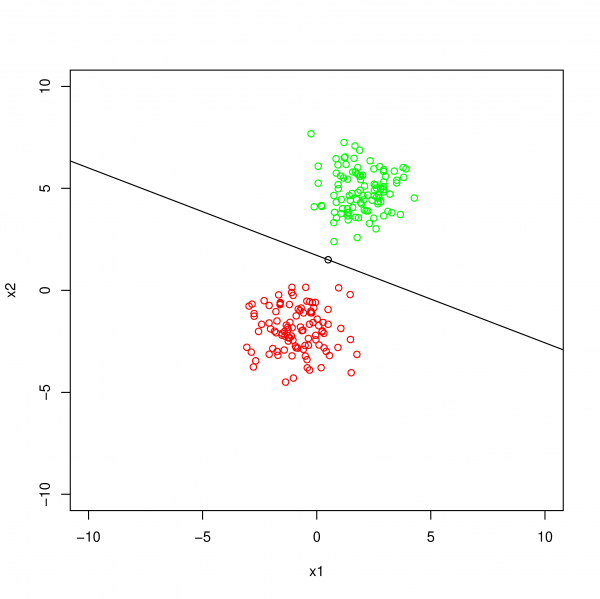Binary Classification Hyperplane

Where as the one-class algorithms are based on recognition since their aim is to recognize data from a particular class, and reject data from all other classes. This is accomplished by creating a boundary that encompasses all the data belonging to the target class within itself, so when a new sample arrives the algorithm only has to check whether it lies within the boundary or outside and accordingly classify the sample as belonging to the target class or the outlier.

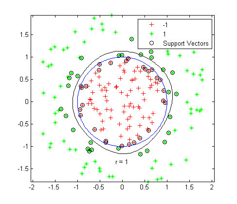One-Class Classification Boundary

Mathematics behind different One-Class Classification Algorithms

In this section, I will explain the mathematics behind different one-class machine learning algorithms by taking a cue from this research paper.

One-Class Gaussian

This is basically a density estimation model. It assumes that the training data are the samples from the Multivariate Normal Population, therefore for a test sample (say z) having n-feaures, the probability of it belonging to the target class can be calculated as follows:

where the parameters μ and Σ are the poputation mean and covariance. Hence, the objective function of this machine learning algorithm is to determine the estimates for μ and Σ. Using the method of maximum likelihood estimator, we can show that the sample mean and sample covariance are the unbiased and consistent estimators for population mean and variance respectively. Hence, once we calculate the probability p(z), we can set a threshold to determine whether a new sample is outlier or not.

One-Class Kmeans

In this method, we first classify the training data into k clusters (which is chosen as per our requirements). Then, for a new sample (say z), the distance d(z) is calculated as the minimum distance of the sample from the centroid of all the k clusters. Now if d(z) is less than a particular thereshold (which is again chosen as per our requirements), then the sample belongs to the target class otherwise it is classified as the outlier.

One-Class K-Nearest Neighbor

Let us take note of some notation before we understand the mathematics behind the algorithm.

d(z,y) : distance between two samples z and y

NN(y) : Nearest Neighbor of sample y

Now given a test sample z, we find the nearest neighbor of z from the training data (which is NN(z) = y) and the nearest neighbor of y (which is NN(y)). Now the rule is to classify z as belonging to the target class when:

where the default value of δ is 1 but can be chosen to satisfy our requirements.

In my next blog entry, I will try to explain the most widely used one-class classification algorithm i.e. one-class support vector machines. Stay tuned !

Thank you very much for making it this far.

One of the most intriguing Machine Learning problems that I have come across was during my 3rd year in the college where a startup named Quantta Analytics presented us with the problem statement about a power distribution company which had observed a significant loss of revenue over a period of time. The loss in revenue was mainly becuase of possible power theft by malicious consumers. The power company resorted to periodic vigilance of customers by sampling and creating a database of only the fraudulent customers to curb this practice. The company wanted the vigilance process to be more robust and effective. Hence, the objective of the problem statement was to deploy a machine learning algorithm to provide a list of customers who are likely to commit fraud. So the problem was effectively a classification problem (with a catch!) where given the attributes of a customer, we had to predict where it is likely to commit the electricity theft or not.

In order to appreciate the problem statement, let us first have the review of the well-known famous classification algorithms. Classification problems try to solve the two or multi-class situation. The goal is to distinguish test data between a number of classes, using training data which has samples from all the possible classes and training data has reasonable level of balance between the various classes. Now the question that arise is - At what levels of imbalance does the use of traditional classifiers becomes futile?

This paper has made observation by conducting experiments on various datasets from the UCI repository, and monitoring the performance of the traditional classifiers. I am listing down the most important observations stated in the paper:

• The performance of the traditional classifiers start to decline when the imbalance between output classes increase and the decline becomes prominent at the ratio 1:2.8.

• At the ratio 1:10, the performance is so poor for traditional classifiers that it can no longer be trusted.

Figure below shows the initial ratio of the classes present in UCI dataset and the ratio at which the performance of the binary classifiers starts to deteriorate.

Now the questions that arise are - what if we have the training data which has imbalance between the classes or data only from one class? Why do we need to study such case? And are there any situations where such data is available?

To answer the latter first, yes there are plenty of situations where we have the data from only one class. Consider a case of a nuclear power plant. We have the measurement of the plant conditions such as temperature, reaction rate when the plant is in working condition. Is it possible to get such measurements in case of an accident? No. Now, if we want to predict the possible scenario of the breakdown of the plant. From the above observations it is sure that the traditional classification algorithms will not perform well. Some other cases are:

• Detection of oil spill

• In computational biology to predict microRNA gene target

There are 2 methods to tackle the case when we have data from only one class:

1. The first method is an obvious approach to generate an artificial second class and proceed with traditional classification algorithms.

2. The second one is to modify the existing classification algoriths to learn on the data from only one class. These algorithms are called "one-class classfication algorithms" and include one-class SVM, One-Class K-Means, One-Class K-Nearest Neighbor, and One-Class Gaussian.

I will be elaborating on the above two methods in my next blog post. Thank you very much for making it this far.

Proposal            Blog            Talk            Presentation            Github

It hasn't been long when I was hugging my friends, calling my parents to inform them of my selection to Google Summer of Code, 2016 program and now here I am writing a wrap-up post for the program. I remember wanting to spend my summers working on the project that involved lots of mathematics, some of the computer science and travel as part of the project. I am so thankful to Google Summer of Code, 2016 program and The Julia Language to have made my each and every wish come true. The thanksgiving note would be incomplete without the mention of my mentors Madeleine and Dj who always helped me whenever I felt like giving up.

Now, coming to the technical aspects of my project, it was divide in 3 phases based on the branches of convex programming namely:

1. Support for complex-domain linear programs

During this phase of the project, I extended the present implementation in Convex.jl to provide support for linear programs involving complex variables and the complex coefficients. The technical details of the implementation are described in the blog post here.

2. Support for second order conic programs

In this phase of the project, I in consulation with my mentors, rewrote many the second order cone atoms such as abs, norm to accept complex arguments. We also had an intense discussion on whether redefining the above atoms to accept complex arguments would violate DCP compliance and we came to a conclusion that defining inverse or the square atoms on complex variables neither makes sense nor does it preserve the DCP compliance.

3. Support for Complex Semidefinite programs

The above 2 phases were relatively difficult for us as we had no literature references and the decision we made were solely based on our understanding and intuition. During this phase, we used the mapping in the introductory section of the research paper here to transform a complex semidefinite program to the corresponding real semidefinite program. Presently, I am writing test cases to check the correctness of our implementation.

The exhaustive list of commits can be found here.

I am glad to have been successfully implemented what I proposed. Presently, I am also writing the documentation and examples to demonstrate the usability of my implementation. The project will culminate with a single pull request to the Convex.jl repository as well as the release of a new version of Convex.jl which we plan to do in next few days.

References

[1].Approximation algorithms for MAX-3-CUT and other problems via complex semidefinite programming

[2].Invariant semidefinite programs

[3].Convex Optimization in Julia

[4].Support for complex variables

[5].Add complex variables